Statistical Analysis

Statistical Analysis of Real-World Operations

Regression, ANOVA, Poisson modeling, and hypothesis testing applied to logistics, manufacturing, and quality control

0.99

Regression R²

p < 0.006

ANOVA (Line Speed)

Industries Analyzed

The Problem

Companies across industries make costly operational decisions based on intuition when rigorous statistical analysis could guide them. A logistics provider needs to know how reliably GDP predicts national shipping costs before expanding into new markets. A soda manufacturer is seeing inconsistent fill levels and needs to isolate whether line speed, carbonation, or their interaction is the root cause before investing in equipment changes. A factory manager must justify whether computer-assisted training is worth the investment over group-based methods, and whether their spring production line actually meets specification targets.

Approach

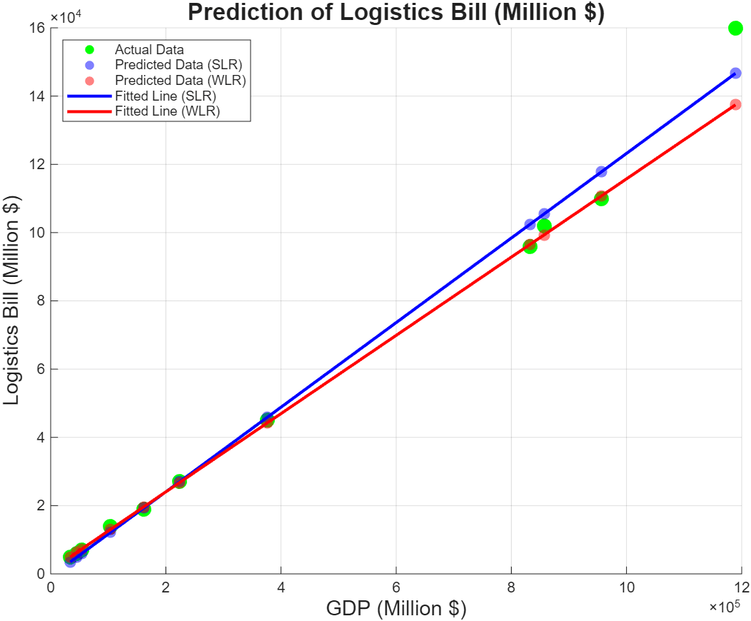
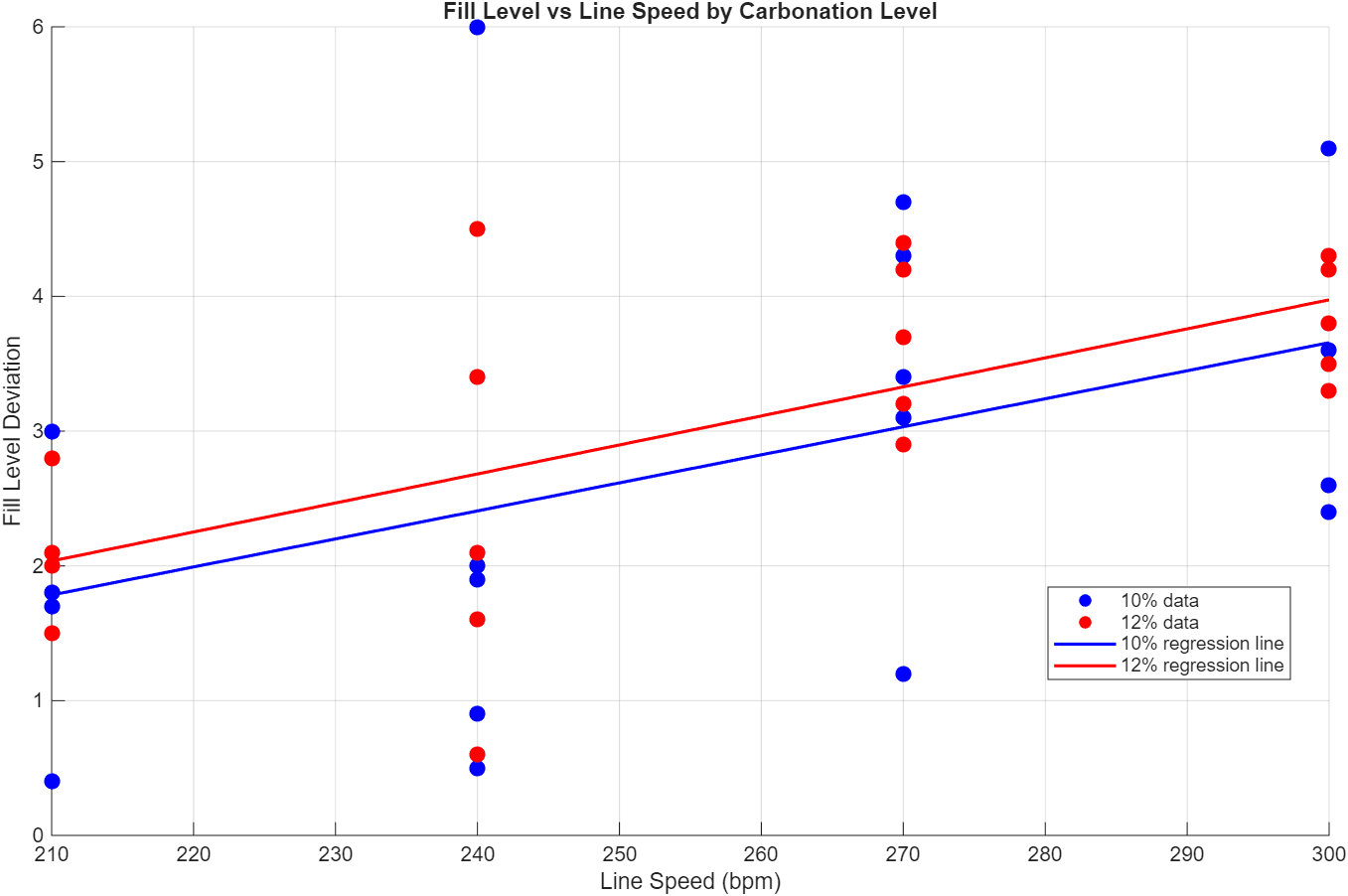
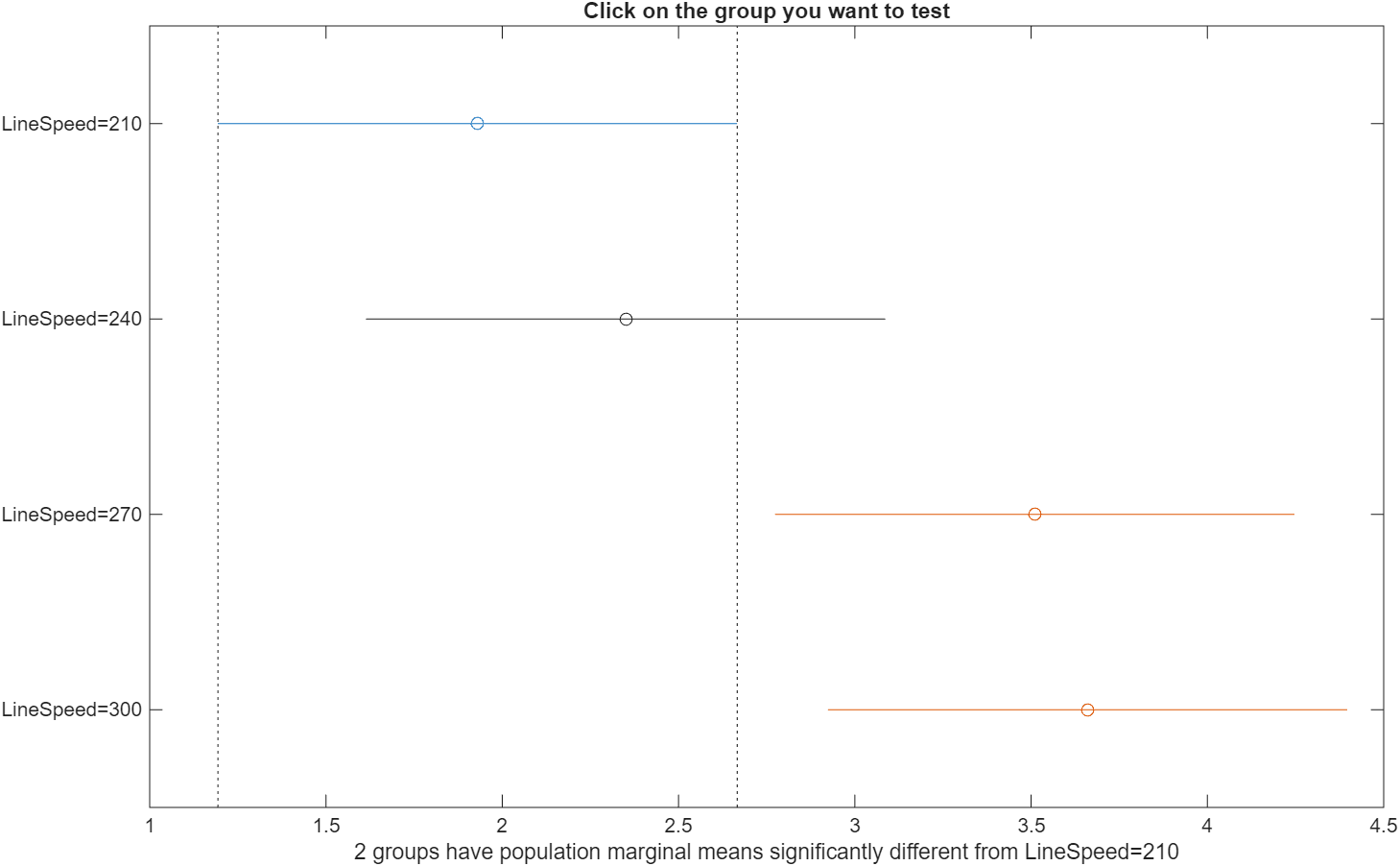
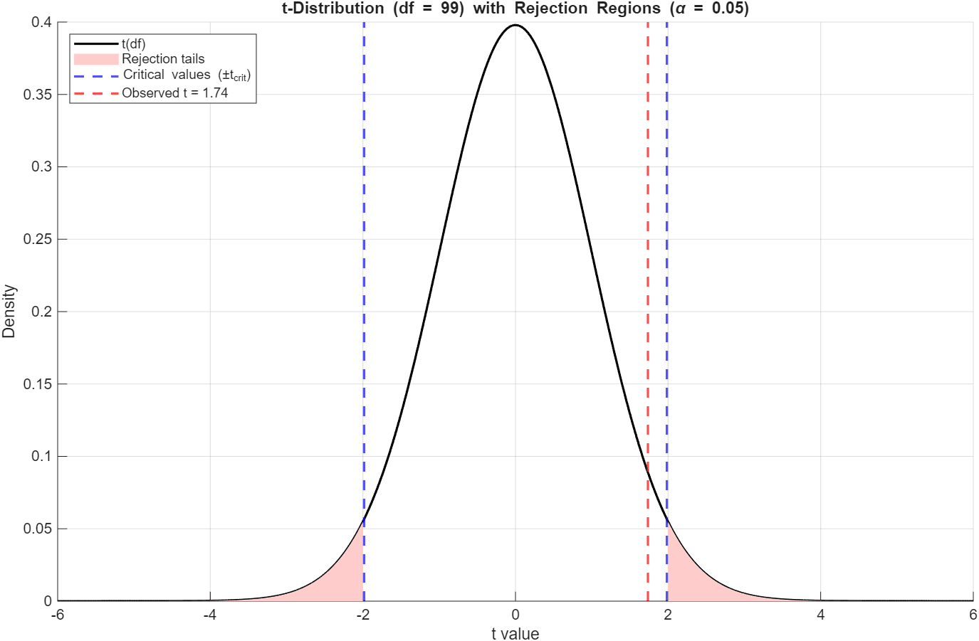
Each domain was treated as a separate statistical investigation with appropriate methods. For the logistics bill problem, simple linear regression was fitted first, followed by residual diagnostics (chi-squared normality test, Breusch-Pagan heteroscedasticity test), then weighted least squares to correct for non-constant variance and produce reliable prediction intervals. For manufacturing, exploratory analysis with correlation testing preceded a two-way ANOVA (4 line speeds x 2 carbonation levels) with Levene's test for equal variance and Tukey post-hoc comparisons to identify which specific speeds drive fill deviations, plus Poisson modeling of equipment breakdowns to inform maintenance staffing. For quality control, F-tests established unequal variance between training groups, leading to Welch's t-test for comparing methods, and normal probability calculations to quantify the out-of-specification rate against tolerances.

Results

The logistics bill regression achieved R² = 0.99, but the Breusch-Pagan test revealed heteroscedasticity (p = 0.009), meaning the simple model's prediction intervals were unreliable at higher GDP values. Switching to WLS corrected this, giving the provider trustworthy cost forecasts for market expansion decisions. The two-way ANOVA pinpointed line speed as the sole significant driver of fill deviation (p = 0.006), with no carbonation effect (p = 0.46) and no interaction (p = 0.999). Tukey post-hoc testing showed speeds 270 and 300 produce significantly higher deviations than 210, giving the manufacturer a clear target for process optimization rather than a blanket equipment overhaul. Poisson modeling revealed an 80.9% chance of 3 or fewer breakdowns per shift but only a 1.1% chance of a breakdown-free day, justifying continuous maintenance staffing. Welch's t-test found no significant difference in mean assembly times (two-sided p = 0.12; one-sided p = 0.06), meaning the training investment cannot yet be justified statistically and a larger trial is needed. The spring process showed a 1.46% out-of-specification rate with the mean not significantly different from the 44 N target (p = 0.086), confirming the line is performing within acceptable bounds.

Figures

Scatter plot comparing SLR and WLS regression lines for logistics bill prediction — Fig. 1 — Comparison of simple linear regression (blue) and weighted least squares (red) fits for logistics bill vs GDP. The WLS fit accounts for heteroscedasticity detected by the Breusch-Pagan test, producing more reliable predictions at higher GDP values.

Scatter plot of fill deviation vs line speed colored by carbonation level with regression lines — Fig. 2 — Fill level deviation vs line speed by carbonation level (10% blue, 12% red) with separate regression lines. The parallel slopes suggest no interaction between carbonation and line speed, confirmed by the ANOVA interaction term (p = 0.999).

Tukey multiple comparison plot showing pairwise differences between line speed groups — Fig. 3 — Tukey post-hoc multiple comparison of mean fill level deviations across line speeds. Line speeds 270 and 300 are significantly different from 210, while 240 is not significantly different from any group.

t-distribution plot with rejection regions and observed test statistic for spring rate test — Fig. 4 — t-distribution for the one-sample t-test on mean spring rate (H₀: μ = 44 N). The observed t-statistic (1.73, red dashed) falls within the acceptance region between the critical values (blue dashed), confirming insufficient evidence to reject the null hypothesis (p = 0.086).